機械学習アルゴリズムの復習(ロジスティック回帰)

ロジスティック回帰による線形クラス分類は、特徴量からクラス分けを行うために使う。

データの用意

method	note
np.random.multivariate_normal([平均], [今日分散], 生成数)	ランダムな多次元正規乱数の生成
train_test_split(x軸, y軸, 分割の割合)	ホールドアウト検証用に各xy配列を訓練用と、検証用に分割

訓練、検証データ作成

from sklearn.model_selection import train_test_split
from sklearn.preprocessing import StandardScaler
import matplotlib.pyplot as plt
import numpy as np
 
np.random.seed(seed=0)
X_0 = np.random.multivariate_normal( [5,5],  [[5,0],[0,5]],  20 ) # [5,5]:平均、[[5,0],[0,5]]：共分散、20：生成する個数
y_0 = np.zeros(len(X_0)) # 0のリストを生成(赤)
 
X_1 = np.random.multivariate_normal( [9,10],  [[6,0],[0,6]],  20 ) # [9,10]:平均、[[6,0],[0,6]]：共分散、20：生成する個数
y_1 = np.ones(len(X_1)) # 1のリストを生成(青)
 
X = np.vstack((X_0, X_1)) # vstack:縦方向に配列を結合
y = np.append(y_0, y_1)
 

X_train, X_test, y_train, y_test = train_test_split(X, y, test_size=0.3)

X_train

array([[ 2.60572435,  7.35782574],
       [11.0987978 ,  8.40531949],
       [ 7.40193187,  9.04236372],
~snip~

y_train

array([0., 1., 1., 1., 0., 1., 1., 0., 1., 1., 0., 0., 0., 1., 1., 1., 0.,
       1., 1., 1., 0., 1., 1., 0., 0., 0., 0., 0., 1., 1., 0., 0., 0., 1.,
       0., 0., 1., 1., 1., 1., 1., 0., 1., 0., 1., 1., 0., 1., 0., 0., 1.,
~snip~

正規化

method	note
StandardScaler()	データの標準化をやるクラス(データの平均や、標準偏差など)
sc.fit_transform()	変換式の計算と変換式を使ったデータ変換を行う

データセットを標準化

# 特徴データを標準化(平均 0、標準偏差 1)
sc = StandardScaler()
X_train_std = sc.fit_transform(X_train) # fit と transform をまとめて行う
X_test_std = sc.transform(X_test) # fitの結果を使ってデータ変換

X_train_std

array([[-1.43501522, -0.15974167],
       [ 1.53555855,  0.17214758],
       [ 0.24252688,  0.37398948],
~snip~

X_test_std

array([[ 1.46270099e+00,  1.31652928e+00],
       [ 1.14335461e+00, -1.47439949e+00],
       [-1.50884298e+00, -2.68581862e-01],
~snip~

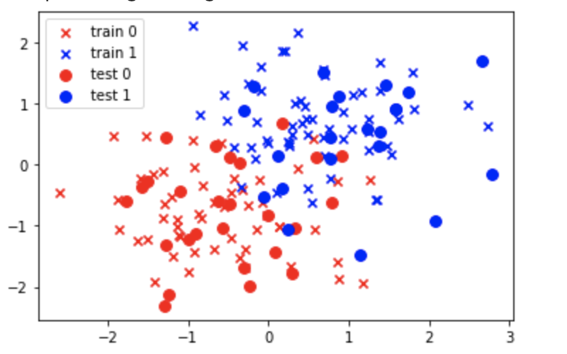
プロット

plt.scatter(X_train_std[y_train==0, 0], X_train_std[y_train==0, 1], c='red', marker='x', label='train 0')
plt.scatter(X_train_std[y_train==1, 0], X_train_std[y_train==1, 1], c='blue', marker='x', label='train 1')
plt.scatter(X_test_std[y_test==0, 0], X_test_std[y_test==0, 1], c='red', marker='o', s=60, label='test 0')
plt.scatter(X_test_std[y_test==1, 0], X_test_std[y_test==1, 1], c='blue', marker='o', s=60, label='test 1')
 
plt.legend(loc='upper left')

学習

from sklearn.linear_model import LogisticRegression # ロジスティック回帰のクラスインポート
 
# 訓練
lr = LogisticRegression()
lr.fit(X_train_std, y_train)

# テストデータ 80個を分類
print (lr.predict(X_test_std))

# 精度を確認
print (lr.score(X_test_std, y_test))

lr.predict(X_test_std)

テストデータを0,1で分類

[1. 0. 0. 0. 1. 1. 0. 0. 0. 1. 1. 1. 1. 0. 1. 0. 0. 1. 0. 0. 1. 0. 0. 1.
 1. 1. 0. 0. 0. 1. 0. 0. 0. 0. 1. 1. 0. 1. 1. 1. 1. 0. 0. 1. 1. 0. 1. 0.]

精度

完全に分類できていない

0.8958333333333334

結果の可視化

# 切片を出力
print (lr.intercept_) 

# 重みを出力
print (lr.coef_) 


w_0 = lr.intercept_[0]
w_1 = lr.coef_[0,0]
w_2 = lr.coef_[0,1]
 
# 重みと切片を使って境界を作る
print(list(map(lambda x: (-w_1 * x - w_0)/w_2, [-2,2])))

# 境界線 プロット
plt.plot([-2,2], list(map(lambda x: (-w_1 * x - w_0)/w_2, [-2,2])))

# データを重ねる
plt.scatter(X_train_std[y_train==0, 0], X_train_std[y_train==0, 1], c='red', marker='x', label='train 0')
plt.scatter(X_train_std[y_train==1, 0], X_train_std[y_train==1, 1], c='blue', marker='x', label='train 1')
plt.scatter(X_test_std[y_test==0, 0], X_test_std[y_test==0, 1], c='red', marker='o', s=60, label='test 0')
plt.scatter(X_test_std[y_test==1, 0], X_test_std[y_test==1, 1], c='blue', marker='o', s=60, label='test 1')
plt.show()

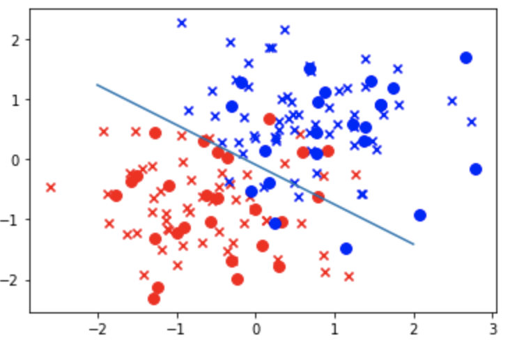
上記の赤と青はランダム関数で設定した平均と分散により位置が変化する。
現状、線形では完全に分類できていないため、精度も 0.8958333333333334 となってしまっている。
線形で綺麗に分類できるデータを作成したい場合は、 np.random.multivariate_normal の引数を調整してやる。
以下は各平均を離してあげることにより綺麗に分類している。

np.random.seed(seed=0)
X_0 = np.random.multivariate_normal( [1,1],  [[5,0],[0,5]],  20 ) # [5,5]:平均、[[5,0],[0,5]]：共分散、20：生成する個数
y_0 = np.zeros(len(X_0)) # 0のリストを生成
 
X_1 = np.random.multivariate_normal( [9,10],  [[6,0],[0,6]],  20 ) # [9,10]:平均、[[6,0],[0,6]]：共分散、20：生成する個数
y_1 = np.ones(len(X_1)) # 1のリストを生成

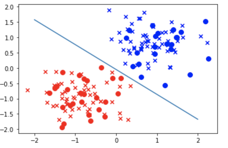
精度も1.0になる
print (lr.score(X_test_std, y_test))

1.0

以上